Intro to LifeCycles

LifeCycles is a python library designed track and analyze the longitudinal evolution of sets (e.g., data clusters, graph communities…)

In this notebook are introduced some of the main features of the library and an overview of its functionalities.

1. Installing LifeCycles

As a first step, we need to make sure that LifeCycles is installed and working.

The library is available for python 3.9, and its stable version can be installed using pip:

!pip install lifecycles

In order to check if LifeCycles has been correctly installed just try to import it

import lifecycles as lcs

2. Creating LifeCycles

LifeCycles allows to represent and analyze the evolution of clusters in time.

As a first step we need to instantiate the LifeCycle object. The object takes the datatype of the clusters’ members as an input.

The default data type is int, but others like str, list and dict are also available.

lc = lcs.LifeCycle(int)

Then, we must add temporally-ordered data partitions. We will generate some random data.

import random
def generate_random_lifecycle(n_snaps=10, max_groups_in_t=7, max_group_size=5, seed=42):
    random.seed(seed)
    snaps = []
    for t in range(5):
        snap_t = [] # snapshot in t
        present_in_t = 0 # entities present in t
        n_groups_t = random.randint(1,max_groups_in_t+1)
        for g in range(n_groups_t):
            size = random.randint(1, max_group_size+1)
            group = list(range(present_in_t, present_in_t+size))
            snap_t.append(group)
            present_in_t += size
        snaps.append(snap_t)
    return snaps

snaps = generate_random_lifecycle()
snaps

[[[0], [1, 2, 3, 4, 5, 6]],
 [[0, 1], [2, 3], [4, 5], [6, 7, 8, 9, 10, 11], [12]],
 [[0, 1, 2, 3, 4], [5, 6, 7, 8]],
 [[0]],
 [[0, 1], [2, 3]]]

# lc.add_partition(snaps[0])   # to add one partition at a time
lc.add_partitions_from(snaps) # to add multiple partitions

When partitions are added, they are automatically assigned a progressive temporal id (integer). The same happens for individual sets, whose id is a string of the form tid_sid, where: - tid is a number indicating temporal id of the partition - sid is a number indicatin the set within that partition

One can retrieve the list of ids as follows:

lc.groups_ids()

['0_0',
 '0_1',
 '1_0',
 '1_1',
 '1_2',
 '1_3',
 '1_4',
 '2_0',
 '2_1',
 '3_0',
 '4_0',
 '4_1']

Basic functionalities include the possibility to get: - the universe set (i.e., the set of unique elements observed across all partitions), - the list of temporal ids associated with each partition, - the elements in a specific set - the set ids associated with a specific partition

list(lc.universe_set())[:10] #  ten elements

[0, 1, 2, 3, 4, 5, 6, 7, 8, 9]

lc.temporal_ids()

[0, 1, 2, 3, 4]

lc.get_group('0_1')

{1, 2, 3, 4, 5, 6}

lc.get_partition_at(0) # returns the group id;
                       # you can get the corresponding group with
                       # lc.get_group(group_id)

['0_0', '0_1']

Another possibility is to remove sets above or below certain thresholds. This allows to reduce noise in the analyses.

lc.filter_on_group_size(min_size=2, max_size=None)

Finally, you can slice the Lifecycle via temporal ids. This method wil return a new object with data in [start, end[ timestamps

sliced = lc.slice(start=0, end=3)
sliced.temporal_ids()

[0, 1, 2]

3. Flows

In this section we provide basic functionalities for anlytical purposes. We start by introducing the concept of group flow.

The idea behind a group’s flow(s) is that a group can contain element that can be allocated in the same/another group in the future. As a group evolves in time, its elements spread to one or multiple groups. So, if a group X_t1 gives elements to groups Y_t2 and Z_t2, its flow towards the future will be described by the elements moving from X_t1 to Y_t2 and from X_t1 to Z_t2. The same holds in the opposite temporal direction, i.e., X_t1 can recieve elements from Y_t0, Z_t0, and so on…

The LifeCycle object allows to easily retrieve the past and future flows of its groups, by specifying group id and temporal direction. Moreover, specifying the min_branch_size parameter restricts the result to those branches (i.e., the collection of elements that move from one group to another, for instance from X_t1 to Y_t2) whose size is equal or above a minimum threshold:

lc.group_flow('2_0', direction='-') # past flow

{'1_0': {0, 1}, '1_1': {2, 3}, '1_2': {4}}

lc.group_flow('2_0', direction='-', min_branch_size=2)

{'1_0': {0, 1}, '1_1': {2, 3}}

Also, the all_flows() method allows to get the past or future flows of all the sets in the LifeCycle:

#lc.all_flows(direction='+', min_branch_size = 19)

3.1. Measures and Events

LifeCycles provides measures to characterize the themporal evolution of groups according to ‘’facets’’. For further details, please refer to the `original paper <>`__.

Note: in the following, - \(X\) identifies the target set that we want to analyze; - \(\mathcal{R}\) identifies the reference partition (i.e., the groups at the previous/next timestamp w.r.t.\(X\)) - \(R\) identifies a group/cluster in \(\mathcal{R}\)

Unicity Facet:

\[\begin{split}\begin{equation} \mathcal{U} = \begin{cases} \frac{|R_1\cap X|-|R_2\cap X|}{|\bigcup_{R \in \mathcal{R}} R|} & \text{if } |\mathcal{R}| \geq 2\\ 1 & \text{otherwise} \end{cases} \end{equation}\end{split}\]

This score guarantees that a large value corresponds to (e.g., in the backward perspective) having one dominating source, and reciprocally, that having a dominating souce leads to a high score. Conversely, having a low score corresponds to having no dominating unique source, and having no dominating source leads to a low score.

Identity Facet:

\[\begin{split}\begin{equation} \label{eq:contr} \mathcal{I} = \begin{cases} \frac{1}{|\bigcup_{R \in \mathcal{R}} R|} \sum_{R \in \mathcal{R}} |R \cap X | \frac{|R \cap X|}{|R|} & \text{if } |\mathcal{R}| > 0\\ 0 & \text{otherwise} \end{cases} \end{equation}\end{split}\]

As an illustrative example, assume that a single set of 10 elements, \(R\), provides elements to \(X\) with two alternative scenarios: a) it provides a single element, and b) it provides 9 out of 10 elements. In the former scenario, the contribution \(\mathcal{I}\) will approach 0; in the latter, it will approach 1 (reaching those extreme values only when none or all elements of \(\mathcal{R}\) are present in \(X\)).

Note that \(\mathcal{I}=0\) if there is no related set: in that case, the group identity is completely lost (forward) or completely new (backward).

Outflow Facet:

\[\begin{equation} \mathcal{O} = \frac{|X - \bigcup_{R \in \mathcal{R}}R|}{|X|} \end{equation}\]

This facet quantifies the fraction of members in \(X\) that are not observed in the previous timestamp, i.e., the new, never-before-seen elements.

These facets can be computed for a group’s past or future flow as follows.

Note that also the size of the group is returned

lcs.analyze_flow(lc, target='2_0', direction='-')

{'U': 0.0, 'I': 0.9, 'O': 0.0, 'size': 5}

complete_flow_analysis = lcs.analyze_all_flows(lc, direction='-') # computes for all flows

Then, it is possible to obtain the event weights as defined in the paper

e_ws = lcs.events_all(lc)
past = e_ws['-'] # or +
fut = e_ws['+']

past['1_0']

{'Birth': 0.4166666666666667,
 'Accumulation': 0.0,
 'Growth': 0.08333333333333333,
 'Expansion': 0.0,
 'Continuation': 0.08333333333333333,
 'Merge': 0.0,
 'Offspring': 0.4166666666666667,
 'Reorganization': 0.0}

3.2. Validation

TO BE REVISED

It is also possible to obtain statistically significant flows only, by comparing them to a null distribution.

#one_validated =  lcs.validated_flow(lc, target='3_3', direction='-', min_branch_size=1,
#                                   num_permutations=1000, significance_level=.05)
validated = lcs.validate_all_flows(lc, direction='-', min_branch_size=1,
                                   iterations=1000)

3.3. Attributes

LifeCycles provides support for studying flows along with element metadata. To attach such metadata to the elements we use the set_attributes method

random.seed(42)
cls = dict()
for e in lc.universe_set():
    cls[e] = random.choice(['red', 'blue'])

from collections import defaultdict
attrs = defaultdict(dict) # {n: {t: 'value', ...}, ...}
for e in lc.universe_set():
    for t in lc.temporal_ids():
        attrs[e][t] = cls[e]

lc.set_attributes(attrs, 'color')

Then, we can retrieve the attributes with a get method

# lc.get_attributes(attr_name='class') # get all attributes for all elements
lc.get_attributes(attr_name='color', of=0) # get attribute of a specific element, by timestamp

{0: 'red', 1: 'red', 2: 'red', 3: 'red', 4: 'red'}

When analyzing flows, adding the attribute as a parameter results in additional information, namely, (i) the entropy of the set w.r.t. the attribute; (ii) the change w.r.t. the past/future average entropy; (iii) the purity ,i.e., the relative frequency of the most frequent attribute value; (iv) the most common attribute value

res = lcs.analyze_flow(lc, target='2_0', direction='-', attr='color')
res

{'U': 0.0,
 'I': 0.9,
 'O': 0.0,
 'size': 5,
 'color_H': 0.7219280948873623,
 'color_H_change': 0.388594761554029,
 'color_purity': 0.8,
 'color_mca': 'red'}

4. Visualization

Lifecycles offers several visualization facilities

lc = lcs.LifeCycle(int)
lc.add_partitions_from(snaps)
lcs.plot_flow(lc,
              slice=(0,4), # slice according to temporal ids
              node_focus=0 # focus on specific nodes (communities will be highlighted)
             )

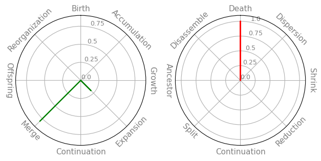
lcs.plot_event_radars(lc, '2_0', min_branch_size=2)

4. IO

To read/write a LifeCycle object on your machine:

# write
filename = 'data/my-lc.json'
lc.write_json(filename)

# read
lc = lcs.LifeCycle()
lc.read_json(filename)

Loaded LifeCycle from data/my-lc.json